Problem

The probability distribution of $X$, the number of imperfections found in every 10 meters of synthetic fabric, is defined as:

$$\begin{array}{|c|c|} \hline X & P(X) \\ \hline 0 & 0.41 \\ 1 & 0.37 \\ 2 & 0.16 \\ 3 & 0.05 \\ 4 & 0.01 \\ \hline \end{array}$$

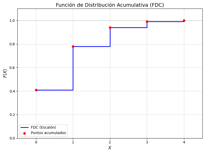
Construct the cumulative distribution function of X and graph it.

Key Concepts

• Discrete random variable: A variable that can take isolated, countable values.
• Probability distribution: Assigns a probability to each possible value of the variable.
• Cumulative distribution function (CDF): Determines the probability that the variable takes a value less than or equal to a given number.

Solution

👉 View solution

Step 1: Verify that the probability distribution is valid

We check that the sum of all probabilities equals 1:

$$\sum_{x=0}^{4} P(X=x) = 0.41 + 0.37 + 0.16 + 0.05 + 0.01 = 1$$

Step 2: Calculate the cumulative distribution function

The cumulative distribution function $F(x)$ is defined as:

$$F(x) = P(X \leq x) = \sum_{t \leq x} P(X = t)$$

We calculate $F(x)$ for each value of $x$:

$$\begin{array}{|c|c|c|} \hline X & P(X) & F(X) \text{ Cumulative} \\ \hline 0 & 0.41 & 0.41 \\ 1 & 0.37 & 0.41 + 0.37 = 0.78 \\ 2 & 0.16 & 0.78 + 0.16 = 0.94 \\ 3 & 0.05 & 0.94 + 0.05 = 0.99 \\ 4 & 0.01 & 0.99 + 0.01 = 1.00 \\ \hline \end{array}$$

Step 3: Express the cumulative distribution function by intervals

The complete cumulative distribution function is expressed as:

$$F(x) = \begin{cases} 0, & x < 0 \\ 0.41, & 0 \leq x < 1 \\ 0.78, & 1 \leq x < 2 \\ 0.94, & 2 \leq x < 3 \\ 0.99, & 3 \leq x < 4 \\ 1, & x \geq 4 \end{cases}$$

Step 4: Graphical representation of the CDF

The cumulative distribution function is a step function that increases discretely at the values of the random variable:

Practical Applications

• Quality control: This type of distribution is used to monitor and control quality in textile manufacturing processes.
• Defect estimation: It allows predicting the probability of finding a specific number of defects in a certain length of material.
• Decision making: It helps decide whether a production batch meets established quality standards.

Conclusion

The cumulative distribution function is an essential tool in statistics for analyzing the behavior of discrete random variables. In this particular case, it allows us to determine the cumulative probability of finding up to a certain number of imperfections in a fabric sample, which is fundamental for quality control processes in the textile industry.